Analyse Results¶

Example on how to analyse Gromacs results of non-equilibrium free energy calculations. For equilibrium results, you can analyse the data with the Gromacs gmx bar command, or with the alchemlyb library.

The data you need for estimating free energy differences is contained in the dgdl.xvg files that Gromacs outputs during a non-equilibrium simulation. The free energy difference can then be estimated using the estimators available in pmx:

In practice, we would recommend to either use BAR or CGI as they are more robust. Furthermore, an advantage of BAR over CGI is that it does not rely on the Gaussian assumption for the distribution of the work values.

To get the free energy estimate, you first need to recover the work values by integrating the data.

>>> from glob import glob
>>> from pmx.analysis import read_dgdl_files
>>> from pmx.estimators import BAR

>>> # get dgdl.xvg files for the forward and reverse transitions
>>> ff = glob('for*.xvg')  # forward
>>> fr = glob('rev*.xvg')  # reverse

>>> # now get integrated work values from them
>>> wf = read_dgdl_files(ff, verbose=False)
>>> wr = read_dgdl_files(fr, verbose=False)

Then, you can use the integrated work values for the estimation of the free energy difference. E.g. for BAR:

>>> # use BAR to estimate the free energy difference
>>> bar = BAR(wf=wf, wr=wr, T=298)
>>> # print estimated dG and its uncertainty
>>> print('%.2f +/- %.2f kJ/mol' % (bar.dg, bar.err))
0.85 +/- 0.56 kJ/mol

Similarly, for the CGI estimator:

>>> cgi = Crooks(wf=wf, wr=wr)
>>> jarz = Jarz(wf=wf, wr=wr, T=298)

>>> # print Crooks estimate
>>> print('%.2f kJ/mol' % cgi.dg)
0.93 kJ/mol

Numerical uncertainty estimates can be obtain by bootstrap, by setting the number of bootstrap samples with the nboots argument.

>>> bar = BAR(wf=wf, wr=wr, T=298, nboots=100)
>>> print('%.2f kJ/mol' % bar.err_boot)
0.66 kJ/mol

The CGI estimator has two types of bootstrapped uncertainties: attributes err_boot1 and err_boot2. The first uses parametric boostrap by resampling a Gaussian fitted to the distribution of work values, while the second uses non-parametric bootstrap by resampling directly the set of work values. Typically, they return similar estimates of the uncertainty.

>>> cgi = Crooks(wf=wf, wr=wr, nboots=100)
>>> print('%.2f kJ/mol' % cgi.err_boot1)
0.77 kJ/mol
>>> print('%.2f kJ/mol' % cgi.err_boot2)
0.82 kJ/mol

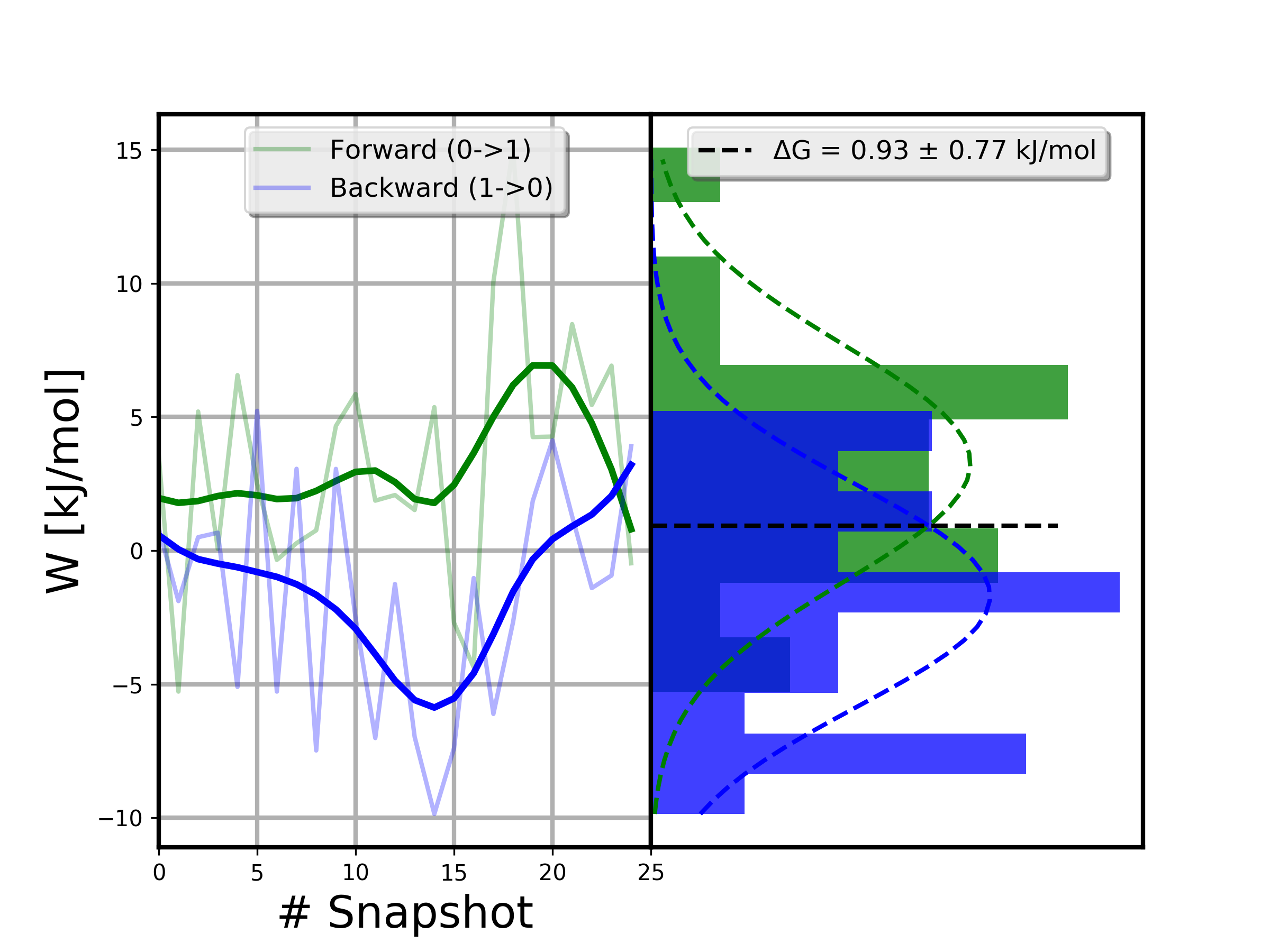
A simple way to inspect the results and identify potential issues with the reliability of the calculations is to plot the distribution of forward and reverse work values.

>>> from pmx.analysis import plot_work_dist
>>> # write distribution plot to 'Wdist.png'
>>> plot_work_dist(wf=wf, wr=wr, nbins=10, dG=cgi.dg, dGerr=cgi.err_boot1)